
MURA
Abstract
Musculoskeletal conditions is one of the most common causes of long term disability affecting 1.7 billion people worldwide, annually leading to 30 million emergency department visits. This paper addresses the problem of automating classifying musculoskeletal radiograph images in remote locations without trained radiologists’ assistance. The classification process can be automated by training a convolutional neural network (CNN) on the MURA data set. The model proposed in this paper achieves an accuracy of .70 and an F1 score of .63.
Introduction
This paper aims to design and implement a deep learning model, trained on the musculoskeletal radiograph images to detect abnormalities, thereby aiding the advancement of automated medical imaging systems providing healthcare access in remote locations with restricted access to trained radiologists.
Modeling
Justification of layer elements
The convolutional neural network (CNN) is a concept introduced by (Fukushima1980), later greatly improved by (Lecun1998) that has significantly impacted computer vision. A CNN is used for pattern detection, where one or more hidden convolution layers uses filters to convolve or scan over an input matrix, such as a binary image. These filters closely resemble neurons in a dense layer, where a filter is learned to detect a specific patter such as an edge or circle; adding more filters to a convolutional layer will enable more features to be learned. The filter size is the size of the matrix convolving over the image matrix, and the stride is the number of pixel shifts over the input matrix. For each stride a matrix multiplication is performed on the image and filter matrix, which results in a feature map as the output. When the filter does not fit the image, two options are available—either dropping the part of the image matrix that does not fit the filter, which is called valid padding, or add zeros to the image matrix’ edges, enabling the filter matrix to fit the image matrix entirely, this is called zero-padding. The most common activation function for a convolutional layer is the Rectified Linear Unit (ReLU) function. ReLU is an activation function with low computational cost since it is almost a linear function. Transforming the input to the maximum of zero or the input value itself makes it converge fast, meaning that the positive linear slope does not saturate or plateau when the input gets large. Unlike sigmoid or than, ReLU does not have a vanishing gradient problem. To reduce the dimensionality of a feature map, that is, the number of tunable parameters, spatial pooling can be applied, which is called subsampling or downsampling. While there are different types of spatial pooling, Max-pooling is often used in CNN’s. A Max-pooling layer operates much like convolutional layers, it also uses filters and stride, but it takes the maximum value in its filter matrix as the output value. A Max-pooling layer with an input matrix of 8x8 with a filter size of 2x2 would have an output of 4x4 containing the larges value for each region. This downsampling will decrease the computational cost for the following layers in the network. This concludes the feature learning part of the CNN and commences with the feature learning part. A convolutional or max-pooling layer outputs a matrix; however, a fully-connected layer only accepts vectors. Therefore, a flattening layer is added to reduce the last convolutional layer’s output dimensionality to shape (-1, 1), or transform the matrix into a vector. Adding a fully-connected layer can be a computationally cheap way of learning non-linear combinations of higher-level features represented by the convolutional or max-pooling layer’s output. Hidden fully-connected layers also called dense layers in a CNN, often use ReLU as their activation function. The final layer, the output layer, is a fully-connected layer with the same number of neurons as classes to be classified. The output layers’ activation function is dependent on the loss function. Using a single neuron sigmoid activated dense layer for the network’s output, compiled with binary cross-entropy as the loss function would yield the same result as using two softmax activated neurons in a network using categorical cross-entropy as the loss function; in other words, a binary classification.
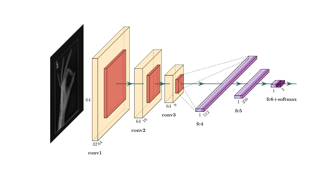
Model architecture
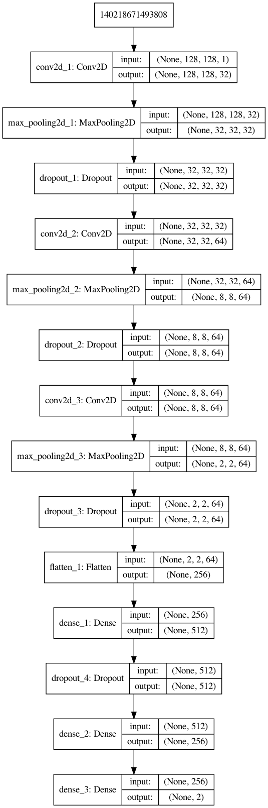
The proposed CNN model is designed to accept N amount of 128x128 image matrices with 1 color channels; it consists of three convolutional layers of 32, 64, and 64 filters, each of filter size 3x3, with zero-padding, and ReLU as the activation function. The first convolutional layer is followed by a max-pooling layer of pool size 4x4, and the last two convolutional layers have a pool size of 2x2, each followed by a dropout layer with a dropout rate of 0.15. A flattening layer is added to transform matrix output to vector inputs to be accepted by the first dense layer, which is comprised of 512 ReLU activated neurons, followed by a dropout layer with a 0.5 dropout rate. The last hidden layer is a dense layer of 256 ReLU activated neurons. The model’s final layer, its output, is a 2 neuron softmax activated dense layer allowing for binary classification. The general architecture of this model is shown in figure 1.
Dataset
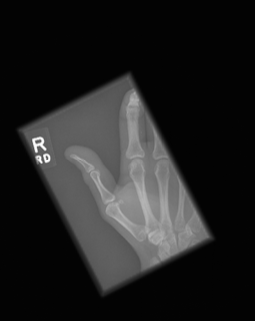
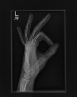
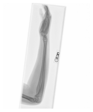
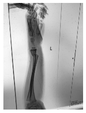
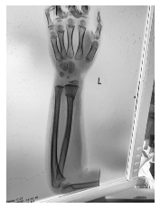
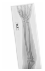
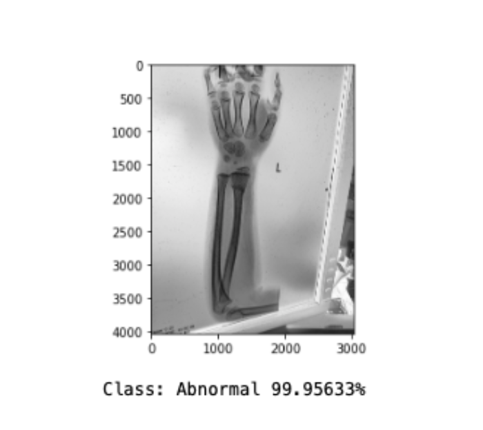
The dataset used to train the CNN model is the publicly available Large Dataset for Abnormality Detection in Musculoskeletal Radiographs, widely known as MURA (Rajpurkar2018). The MURA dataset wast the basis for a Deep Learning competition hosted by Stanford, which expected the participants to detect bone abnormalities. MURA is a dataset of musculoskeletal radiographs consisting of 14,863 studies collected from 12,173 patients, with 40,561 multi-view radiographic images, meaning that one patient can have multiple images used for diagnosis, and seven different categories elbow, finger, forearm, hand, humerus, shoulder, and wrist. Between 2001 and 2012, board-certified radiologists from the Stanford Hospital has manually labeled each study during clinical radiographic interpretation. The dataset images vary in aspect ration and resolution, which can be beneficial during neural network training. The dataset is split into training (11,184 patients, 13,457 studies, 36,808 images), validation (783 patients, 1,199 studies, 3,197 images), and test (206 patients, 207 studies, 556 images), and there is no overlap in patients between any of the sets. The test set is not available to the general public; therefore, in preparation for training the model, the training set is further split into a new train 80% and a validation set 20%, keeping the test set for evaluation after model training. The reasoning for this decision is to be able to present the models’ generalization ability and accuracy. Figure \ref{fig:images} shows example images of a normal figure 2 and an abnormal figure figure 3 diagnosis.
Experimental setup
For model development and training of the model, Google’s open-source python library Keras is used as an interface to the machine learning library TensorFlow. A sequential model is defined using the Keras API with the layered architecture described in the modeling section. The model is compiled with the stochastic gradient descent variant Adam, an adaptive learning rate optimization algorithm specifically designed for deep neural network training (Kingma2017). Categorical cross-entropy is used as the loss function, using accuracy as the evaluation metric. The model training is set to feed batches of 32 image arrays for 50 epochs, with an initial learning rate of .001. However, to find the optimal learning rate, the ReduceLROnPlateau method reduces the learning rate with a factor of .5 if val_loss does not decrease for two epochs. The EarlyStopping method is also implemented to keep from running if val_loss does not decrease for five epochs.
Discussion
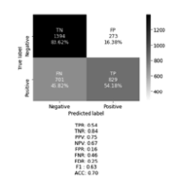
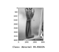
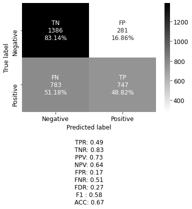
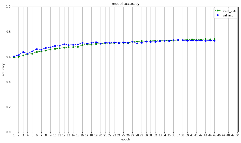
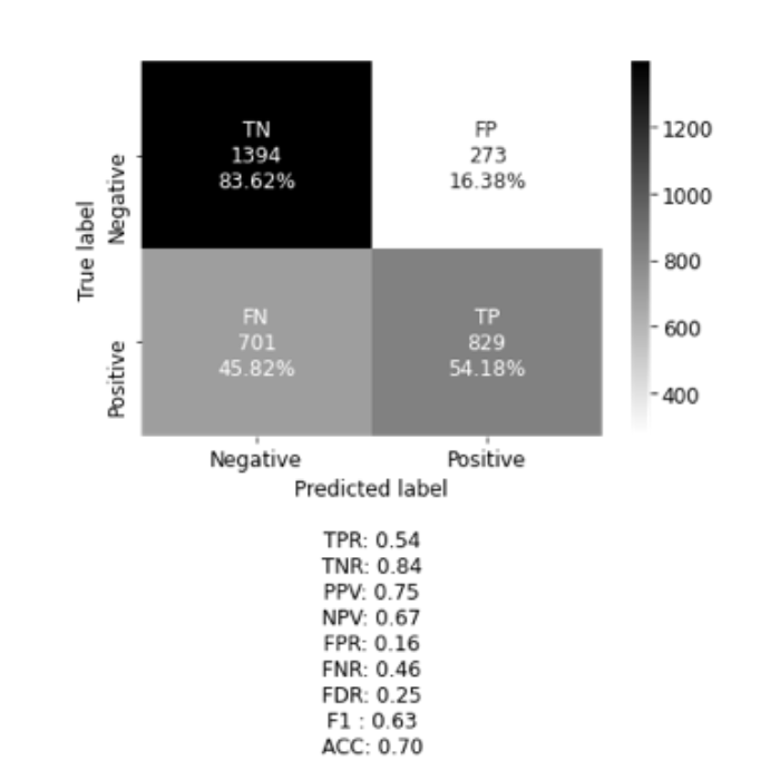
Overfitting is a common problem in deep neural networks. To combat this problem, several measures can be taken. The first choice is to increase the amount of training data. If this is not possible, data augmentation like mirroring, cropping, rotating, or embossing can be performed on the available data to provide additional training scores. However, this method did not increase the accuracy of this model. In the experimental stage of model development batch normalization, as well as L1, and L2 regularization, were implemented without improving performance. Yet, regularization by adding dropout proved to be significant in decreasing overfitting. The next challenge was the model would seem to settle to local minima, and essentially stop training. To rectify this, the Nadam optimizer was implemented, which is the Adam optimizer with Nesterov momentum. Many decay rates were tested without bearing fruit, thereby returning to the original optimizer. The best result of the final model achieved an overall accuracy score of .70, and F1 score of .63, which is the harmonic mean of the precision (positive predictive value) and sensitivity (true positive rate). In this case, it is important to have a low number of false-negative (FN) classifications. The proposed model has a false-negative classification of 45.82\%, as shown in figure 4, making it too unreliable to go into production. The model is, however, capable of making the correct prediction of personal test image as shown in figure 5.
Conclusion
A convolutional neural network has been designed, implemented, and trained on musculoskeletal radiograph images from the MURA dataset to classify bone abnormalities. The proposed model achieved an overall accuracy score of .70, and F1 score of .63. The model did not achieve a high enough accuracy to go into production; further research is needed.
Jupyter Notebook
Note! After finishing this assessment in my ML course, I understood that I should not have augmented the whole dataset, but rather the abnormal cases. What you see below is what I submitted, and the augmentation should be altered to give a better performance.
import os
os.environ["KERAS_BACKEND"] = "plaidml.keras.backend"

import numpy as np
import pandas as pd
import matplotlib.pyplot as plt
import seaborn as sns
import cv2
import csv
import time
import gc

from keras.models import Sequential, Model, load_model
from keras.layers import Dense, Conv2D, MaxPooling2D, Flatten, Dropout, ZeroPadding2D, BatchNormalization, Activation, MaxPool2D, GlobalAveragePooling2D, SeparableConv2D
from keras import Input
from keras.optimizers import Adam, Nadam
from keras.utils import to_categorical, plot_model
from keras.callbacks import ModelCheckpoint, EarlyStopping, ReduceLROnPlateau
from keras.preprocessing.image import img_to_array, load_img

from keras_sequential_ascii import keras2ascii

from ann_visualizer.visualize import ann_viz

from IPython.display import Image

from sklearn.metrics import confusion_matrix
from sklearn.model_selection import train_test_split

from albumentations import (
    HorizontalFlip, IAAPerspective, ShiftScaleRotate, CLAHE, RandomRotate90,
    Transpose, ShiftScaleRotate, Blur, OpticalDistortion, GridDistortion, HueSaturationValue,
    IAAAdditiveGaussianNoise, GaussNoise, MotionBlur, MedianBlur, IAAPiecewiseAffine,
    IAASharpen, IAAEmboss, RandomBrightnessContrast, Flip, OneOf, Compose
)

#np.set_printoptions(suppress=True)
%matplotlib inline
Using plaidml.keras.backend backend.
def csv_reader_parser(filepath):
    df = pd.read_csv(filepath, dtype=str, header=None)
    df.columns = ["image_path"]

    df["label"] = df["image_path"].map(lambda x:1 if "positive" in x else 0)
    df["category"]  = df["image_path"].apply(lambda x: x.split("/")[2])
    df["patient_id"]  = df["image_path"].apply(lambda x: x.split("/")[3].replace("patient",""))

    return df
def augmentor(p=0.5):
    return Compose([
        RandomRotate90(),
        Flip(),
        Transpose(),
        OneOf([
            IAAAdditiveGaussianNoise(),
            GaussNoise(),
        ], p=0.2),
        OneOf([
            MotionBlur(p=0.2),
            MedianBlur(blur_limit=3, p=0.1),
            Blur(blur_limit=3, p=0.1),
        ], p=0.2),
        ShiftScaleRotate(shift_limit=0.0625, scale_limit=0.2, rotate_limit=45, p=0.2),
        OneOf([
            OpticalDistortion(p=0.3),
            GridDistortion(p=0.1),
            IAAPiecewiseAffine(p=0.3),
        ], p=0.2),
        OneOf([
            CLAHE(clip_limit=2),
            IAASharpen(),
            IAAEmboss(),
            RandomBrightnessContrast(),
        ], p=0.3),
        HueSaturationValue(p=0),
    ], p=p)
def image_processor(dir_name, path_csv, shape=(128, 128), colour=0, scale=False, augment=False):

    data = []
    transform = augmentor()

    # open the csv file containing the image paths
    with open(path_csv, "r") as path:
        # read all the paths from the CSV file
        imagepaths = csv.reader(path)
        # loop over the images paths
        for imagepath in imagepaths:
            # create a complete path for an image based on it location on my pc
            imagepath = os.path.join(dir_name, imagepath[0])
            # read the image as grayscale image, 0=grayscale, 1=colour image, -1=unchanged
            image = cv2.imread(imagepath, colour)
            # resize the to 128 x 128, you can choose the image size you want here
            image = cv2.resize(image, shape)
            # creates a training data in matrix form of all the raw pixel values
            data.append(image)
            if augment:
                augmented_image = transform(image=image)['image']
                data.append(augmented_image)

    if scale:
        # scale the raw pixel intensities to the range [0, 1]
        data = np.array(data, dtype="float") / 255.0

    return data
def pickler(filename, operation, data=""):
    import pickle
    if operation == "save":
        pickle_out = open(f"{filename}.pickle", "wb")
        pickle.dump(data, pickle_out)
        pickle_out.close()
    elif operation == "load":
        pickle_in = open(f"{filename}.pickle", "rb")
        data = pickle.load(pickle_in)

    return data
def cm_plot(y_test,
            y_pred,
            categories=None,
            cmap="binary",
            cbar=True,
            figsize=None,
            calculate=False,
            legend=False):

    cf_matrix = confusion_matrix(y_test_expt, y_pred)
    cf_matrix_normal = cf_matrix.astype('float') / cf_matrix.sum(axis=1)[:, np.newaxis]

    if categories is None:
        categories = [0, 1]

    # Code to generate text inside each square
    group_names = ["TN", "FP", "FN", "TP"]

    group_counts = ["{0:0.0f}".format(value) for value in
                    cf_matrix.flatten()]

    group_percentages = ["{0:.2%}".format(value) for value in
                         cf_matrix_normal.flatten()]

    labels = [f"{v1}\n{v2}\n{v3}" for v1, v2, v3 in
              zip(group_names, group_counts, group_percentages)]

    labels = np.asarray(labels).reshape(2, 2)

    stats_text = ""

    if calculate:
        # Metrics for Binary Confusion Matrices
        TP = (np.diag(cf_matrix))[1]
        FN = (cf_matrix.sum(axis=1) - np.diag(cf_matrix))[1]
        FP = (cf_matrix.sum(axis=0) - np.diag(cf_matrix))[1]
        TN = cf_matrix.sum() - (FP + FN + TP)
        # Sensitivity, hit rate, recall, or true positive rate
        TPR = TP/(TP+FN)
        # Specificity or true negative rate
        TNR = TN/(TN+FP)
        # Precision or positive predictive value
        PPV = TP/(TP+FP)
        # Negative predictive value
        NPV = TN/(TN+FN)
        # Fall out or false positive rate
        FPR = FP/(FP+TN)
        # False negative rate
        FNR = FN/(TP+FN)
        # False discovery rate
        FDR = FP/(TP+FP)
        # F1 score is the harmonic mean of precision and recall
        F1 = 2 * (PPV * TPR)/(PPV + TPR)
        # Overall accuracy
        ACC = (TP+TN)/(TP+FP+FN+TN)

        if legend:
            print(f"""
                # True Positive
                TP = np.diag(cf_matrix) : {TP:.2f}

                # False Negative, Type II Error
                FN = cf_matrix.sum(axis=1) - np.diag(cf_matrix) : {FN:.2f}

                # False Positive, Type I Error
                FP = cf_matrix.sum(axis=0) - np.diag(cf_matrix) : {FP:.2f}

                # True Negative
                TN = cf_matrix.sum() - (FP + FN + TP) : {TN:.2f}

                # Sensitivity, hit rate, recall, or true positive rate
                TPR = TP/(TP+FN) : {TPR:.2f}

                # Specificity, true negative rate or negative recall
                TNR = TN/(TN+FP) : {TNR:.2f}

                # Precision or positive predictive value
                PPV = TP/(TP+FP) : {PPV:.2f}

                # Negative predictive value
                NPV = TN/(TN+FN) : {NPV:.2f}

                # Fall out or false positive rate
                FPR = FP/(FP+TN) : {FPR:.2f}

                # False negative rate
                FNR = FN/(TP+FN) : {FNR:.2f}

                # False discovery rate
                FDR = FP/(TP+FP) : {FDR:.2f}

                # F1 score is the harmonic mean of positive predictive value
                #  and sensitivity
                F1 = 2 * (PPV * TPR)/(PPV + TPR) : {F1:.2f}

                # Overall accuracy
                ACC = (TP+TN)/(TP+FP+FN+TN) : {ACC:.2f}
                """)

        stats_text = f"\n"\
            f"TPR: {TPR:.2f}\n"\
            f"TNR: {TNR:.2f}\n"\
            f"PPV: {PPV:.2f}\n"\
            f"NPV: {NPV:.2f}\n"\
            f"FPR: {FPR:.2f}\n"\
            f"FNR: {FNR:.2f}\n"\
            f"FDR: {FDR:.2f}\n"\
            f"F1 : {F1:.2f}\n"\
            f"ACC: {ACC:.2f}"

    if figsize is None:
        # Get default figure size if not set
        figsize = plt.rcParams.get("figure.figsize")
    else:
        plt.figure(figsize=figsize)

    font_size = 12

    ax = sns.heatmap(cf_matrix, annot=labels, annot_kws={"size": font_size},
                     fmt="", cmap=cmap, cbar=cbar, xticklabels=categories,
                     yticklabels=categories)

    ax.set_xticklabels(ax.get_xticklabels(), fontsize=font_size)
    ax.set_yticklabels(ax.get_yticklabels(), fontsize=font_size)

    cbar = ax.collections[0].colorbar
    cbar.ax.tick_params(labelsize=font_size)

    plt.ylabel("True label", fontsize=font_size)
    plt.xlabel("Predicted label\n" + stats_text, fontsize=font_size)
    plt.show()
def data_setup(dir_name, train_path, teat_path, preprocessed=True, shape=(128, 128), binary=False, augment=False):
    if preprocessed:
        print("[INFO] Loading preprocessed file(s)")
        X_train = pickler("X_train", "load")
        y_train = pickler("y_train", "load")
        X_test = pickler("X_test", "load")
        y_test = pickler("y_test", "load")

        if binary:
            binary = False
            print("[INFO] Can only be used on dataload")
            y_test_expt = y_test
        else:
            y_test_expt = np.array([y_test[x][1] for x in range(len(y_test))], dtype=int)

    else:
        train_image_paths_csv = "MURA/MURA-v1.1/train_image_paths.csv"
        test_image_paths_csv = "MURA/MURA-v1.1/valid_image_paths.csv"

        print("[INFO] Loading images from CSV filepaths")
        X_train = image_processor("MURA", train_image_paths_csv, shape=shape, scale=True, augment=augment)
        X_test = image_processor("MURA", test_image_paths_csv, shape=shape, scale=True)

        print(f"[INFO] Reshaping images to {shape}")
        X_train = X_train.reshape((X_train.shape[0], *shape, 1))
        X_test = X_test.reshape((X_test.shape[0], *shape, 1))

        train_image_paths = csv_reader_parser(train_image_paths_csv)
        test_image_paths = csv_reader_parser(test_image_paths_csv)

        temp_y_train = np.array([])

        if binary:
            y_train = train_image_paths.label.values
            y_test = test_image_paths.label.values
            if augment:
                temp_y_test = np.array([], dtype="float32")
                for i in range(len(y_train)):
                    temp_y_train = np.append(temp_y_train, [y_train[i]])
                    temp_y_train = np.append(temp_y_train, [y_train[i]])
                temp_y_train = temp_y_train.reshape(-1,2)

                y_train = temp_y_train
            y_test_expt = y_test

        else:
            y_train = to_categorical(train_image_paths.label.values)
            y_test = to_categorical(test_image_paths.label.values)
            if augment:
                temp_y_test = np.array([], dtype="float32")
                for i in range(len(y_train)):
                    temp_y_train = np.append(temp_y_train, [y_train[i]])
                    temp_y_train = np.append(temp_y_train, [y_train[i]])
                temp_y_train = temp_y_train.reshape(-1,2)

                y_train = temp_y_train
            y_test_expt = np.array([y_test[x][1] for x in range(len(y_test))], dtype=int)

        print("[INFO] Saving to preprocessed file(s)")
        X_train = pickler("X_train", "save", X_train)
        y_train = pickler("y_train", "save", y_train)
        X_test = pickler("X_test", "save", X_test)
        y_test = pickler("y_test", "save", y_test)

        # Garbage collection
        del train_image_paths_csv
        del test_image_paths_csv
        del train_image_paths
        del test_image_paths
        gc.collect()

    print("[INFO] Done!")
    return X_train, y_train, X_test, y_test, y_test_expt
def prepare_img(filepath, show=True, img_size = (128, 128)):
    img_array = cv2.imread(filepath, cv2.IMREAD_GRAYSCALE)
    new_array = cv2.resize(img_array, img_size)

    if show:
        plt.imshow(img_array, cmap="Greys")
        plt.axis("off")
        plt.show()

    return new_array.reshape(-1, *img_size, 1)
X_train, y_train, X_test, y_test, y_test_expt = data_setup(
    "MURA",
    "MURA/MURA-v1.1/train_image_paths.csv",
    "MURA/MURA-v1.1/valid_image_paths.csv",
    preprocessed=True,
    shape=(128,128),
    binary=False,
    augment=False
)
[INFO] Loading images from CSV filepaths
[INFO] Reshaping images to (128, 128)
[INFO] Saving to preprocessed file(s)
[INFO] Done!
display(X_train.shape)
display(y_train.shape)
display(X_test.shape)
display(y_test.shape)
display(y_test_expt.shape)
(36808, 128, 128, 1)


(36808, 2)


(3197, 128, 128, 1)


(3197, 2)


(3197,)
from keras.backend import clear_session
clear_session()
# Collective hyperparameters
epochs = 50
batch_size = 32  # Should be a factor of 2.
validation_split = 0.1

learning_rate = .001
learning_rate_reduction_factor = 0.5
learning_rate_min = 0.000001
learning_rate_patience = 2

#b1 = 0.09
#b2 = 0.9995
#epsi = 1e-07

early_stop_patience = epochs/10  # How many times in a row.

# optimizer = Nadam(lr=learning_rate, beta_1=b1, beta_2=b2, epsilon=epsi)
optimizer = Adam(lr=learning_rate)
loss_function = "categorical_crossentropy"
metrics = ["accuracy"]

categories = ["Normal", "Abnormal"]
INFO:plaidml:Opening device "metal_amd_radeon_pro_560.0"
checkpoint_filepath = "checkpoint"

model_checkpoint = ModelCheckpoint(
    filepath=checkpoint_filepath,
    save_weights_only=False,
    monitor="val_loss",
    verbose=1,
    mode="auto",
    save_best_only=True)

lr_reduce = ReduceLROnPlateau(
    monitor="val_loss",
    factor=learning_rate_reduction_factor,
    min_lr=learning_rate_min,
    patience=3,
    verbose=1,
    mode="auto")

early_stop = EarlyStopping(
    monitor="val_loss",
    patience=early_stop_patience,
    mode="auto",
    verbose=1)
    # min_delta=0.1,
# Split into training and validation set
X_train, X_val, y_train, y_val = train_test_split(X_train, y_train, test_size=validation_split, random_state=42)
X_train.shape[1:]
(128, 128, 1)
model = Sequential()

# the 2 first values in in input shape is the width and height of the image, the last is the color channel.
first_layer = X_train.shape[1:]  # <-- Not hidden, not counted

# ### Conv2D ###
# filters is the number of filters that is learning.
# The kernel_size is the filter/matrix size
# The stride is the actual convolving.
# padding = "same" keeps the origional dimensionality

model.add(Conv2D(32, kernel_size=(3,3), activation="relu", padding="same", input_shape=first_layer))
model.add(MaxPooling2D(pool_size=(4,4)))
model.add(Dropout(0.15))

model.add(Conv2D(64, kernel_size=(3,3), activation="relu", padding="same"))
model.add(MaxPooling2D(pool_size=(2,2)))
model.add(Dropout(0.15))

model.add(Conv2D(64, kernel_size=(3,3), activation="relu", padding="same"))
model.add(MaxPooling2D(pool_size=(2,2)))
model.add(Dropout(0.15))

# First dense layer in model has to have a flatten
model.add(Flatten())

model.add(Dense(512, activation="relu"))
model.add(Dropout(0.5))

# Dropout should not be added to last hidden layer
model.add(Dense(256, activation="relu"))

### Will give same result ###
## Binary only
# When using loss="binary_crossentropy"
# model.add(Dense(1, activation="sigmoid"))

## Can also be used when more than two classes
# When using loss="categorical_crossentropy"
model.add(Dense(2, activation="softmax"))
model.compile(optimizer, loss=loss_function, metrics=metrics)
# history = model.fit(X_train, y_train, batch_size=batch_size, epochs=epochs, validation_split=validation_split, verbose=2, callbacks = [model_checkpoint, lr_reduce, early_stop])

history = model.fit(X_train, y_train, batch_size=batch_size, epochs=epochs, validation_data=(X_val, y_val), verbose=2, callbacks = [model_checkpoint, lr_reduce, early_stop])
Train on 33127 samples, validate on 3681 samples
Epoch 1/50
 - 94s - loss: 0.6663 - acc: 0.5940 - val_loss: 0.6512 - val_acc: 0.6039

Epoch 00001: val_loss improved from inf to 0.65118, saving model to checkpoint
Epoch 2/50
 - 88s - loss: 0.6558 - acc: 0.5996 - val_loss: 0.6479 - val_acc: 0.6134

Epoch 00002: val_loss improved from 0.65118 to 0.64794, saving model to checkpoint
Epoch 3/50
 - 87s - loss: 0.6507 - acc: 0.6105 - val_loss: 0.6390 - val_acc: 0.6387

Epoch 00003: val_loss improved from 0.64794 to 0.63904, saving model to checkpoint
Epoch 4/50
 - 88s - loss: 0.6429 - acc: 0.6215 - val_loss: 0.6435 - val_acc: 0.6248

Epoch 00004: val_loss did not improve from 0.63904
Epoch 5/50
 - 88s - loss: 0.6380 - acc: 0.6250 - val_loss: 0.6341 - val_acc: 0.6425

Epoch 00005: val_loss improved from 0.63904 to 0.63407, saving model to checkpoint
Epoch 6/50
 - 88s - loss: 0.6292 - acc: 0.6391 - val_loss: 0.6150 - val_acc: 0.6620

Epoch 00006: val_loss improved from 0.63407 to 0.61499, saving model to checkpoint
Epoch 7/50
 - 88s - loss: 0.6256 - acc: 0.6431 - val_loss: 0.6141 - val_acc: 0.6580

Epoch 00007: val_loss improved from 0.61499 to 0.61406, saving model to checkpoint
Epoch 8/50
 - 88s - loss: 0.6160 - acc: 0.6501 - val_loss: 0.6054 - val_acc: 0.6710

Epoch 00008: val_loss improved from 0.61406 to 0.60545, saving model to checkpoint
Epoch 9/50
 - 89s - loss: 0.6112 - acc: 0.6596 - val_loss: 0.6013 - val_acc: 0.6759

Epoch 00009: val_loss improved from 0.60545 to 0.60129, saving model to checkpoint
Epoch 10/50
 - 89s - loss: 0.6056 - acc: 0.6639 - val_loss: 0.6040 - val_acc: 0.6873

Epoch 00010: val_loss did not improve from 0.60129
Epoch 11/50
 - 88s - loss: 0.6020 - acc: 0.6677 - val_loss: 0.5869 - val_acc: 0.6887

Epoch 00011: val_loss improved from 0.60129 to 0.58687, saving model to checkpoint
Epoch 12/50
 - 88s - loss: 0.5978 - acc: 0.6728 - val_loss: 0.5792 - val_acc: 0.7012

Epoch 00012: val_loss improved from 0.58687 to 0.57915, saving model to checkpoint
Epoch 13/50
 - 88s - loss: 0.5945 - acc: 0.6768 - val_loss: 0.5823 - val_acc: 0.6946

Epoch 00013: val_loss did not improve from 0.57915
Epoch 14/50
 - 89s - loss: 0.5915 - acc: 0.6786 - val_loss: 0.5795 - val_acc: 0.6960

Epoch 00014: val_loss did not improve from 0.57915
Epoch 15/50
 - 89s - loss: 0.5886 - acc: 0.6807 - val_loss: 0.5823 - val_acc: 0.6979

Epoch 00015: val_loss did not improve from 0.57915

Epoch 00015: ReduceLROnPlateau reducing learning rate to 0.0005000000237487257.
Epoch 16/50
 - 89s - loss: 0.5757 - acc: 0.6929 - val_loss: 0.5628 - val_acc: 0.7118

Epoch 00016: val_loss improved from 0.57915 to 0.56285, saving model to checkpoint
Epoch 17/50
 - 89s - loss: 0.5685 - acc: 0.6996 - val_loss: 0.5671 - val_acc: 0.7050

Epoch 00017: val_loss did not improve from 0.56285
Epoch 18/50
 - 88s - loss: 0.5693 - acc: 0.6992 - val_loss: 0.5641 - val_acc: 0.7120

Epoch 00018: val_loss did not improve from 0.56285
Epoch 19/50
 - 88s - loss: 0.5645 - acc: 0.7025 - val_loss: 0.5618 - val_acc: 0.7175

Epoch 00019: val_loss improved from 0.56285 to 0.56182, saving model to checkpoint
Epoch 20/50
 - 88s - loss: 0.5615 - acc: 0.7046 - val_loss: 0.5642 - val_acc: 0.7063

Epoch 00020: val_loss did not improve from 0.56182
Epoch 21/50
 - 88s - loss: 0.5597 - acc: 0.7084 - val_loss: 0.5615 - val_acc: 0.7131

Epoch 00021: val_loss improved from 0.56182 to 0.56148, saving model to checkpoint
Epoch 22/50
 - 88s - loss: 0.5583 - acc: 0.7073 - val_loss: 0.5612 - val_acc: 0.7112

Epoch 00022: val_loss improved from 0.56148 to 0.56124, saving model to checkpoint
Epoch 23/50
 - 87s - loss: 0.5571 - acc: 0.7099 - val_loss: 0.5597 - val_acc: 0.7153

Epoch 00023: val_loss improved from 0.56124 to 0.55966, saving model to checkpoint
Epoch 24/50
 - 88s - loss: 0.5545 - acc: 0.7100 - val_loss: 0.5637 - val_acc: 0.7096

Epoch 00024: val_loss did not improve from 0.55966
Epoch 25/50
 - 88s - loss: 0.5545 - acc: 0.7094 - val_loss: 0.5628 - val_acc: 0.7137

Epoch 00025: val_loss did not improve from 0.55966
Epoch 26/50
 - 88s - loss: 0.5533 - acc: 0.7088 - val_loss: 0.5605 - val_acc: 0.7134

Epoch 00026: val_loss did not improve from 0.55966

Epoch 00026: ReduceLROnPlateau reducing learning rate to 0.0002500000118743628.
Epoch 27/50
 - 87s - loss: 0.5421 - acc: 0.7214 - val_loss: 0.5514 - val_acc: 0.7213

Epoch 00027: val_loss improved from 0.55966 to 0.55136, saving model to checkpoint
Epoch 28/50
 - 87s - loss: 0.5403 - acc: 0.7210 - val_loss: 0.5595 - val_acc: 0.7077

Epoch 00028: val_loss did not improve from 0.55136
Epoch 29/50
 - 87s - loss: 0.5374 - acc: 0.7252 - val_loss: 0.5567 - val_acc: 0.7134

Epoch 00029: val_loss did not improve from 0.55136
Epoch 30/50
 - 88s - loss: 0.5362 - acc: 0.7242 - val_loss: 0.5485 - val_acc: 0.7226

Epoch 00030: val_loss improved from 0.55136 to 0.54848, saving model to checkpoint
Epoch 31/50
 - 89s - loss: 0.5335 - acc: 0.7273 - val_loss: 0.5520 - val_acc: 0.7194

Epoch 00031: val_loss did not improve from 0.54848
Epoch 32/50
 - 89s - loss: 0.5341 - acc: 0.7287 - val_loss: 0.5503 - val_acc: 0.7196

Epoch 00032: val_loss did not improve from 0.54848
Epoch 33/50
 - 88s - loss: 0.5328 - acc: 0.7274 - val_loss: 0.5481 - val_acc: 0.7264

Epoch 00033: val_loss improved from 0.54848 to 0.54807, saving model to checkpoint
Epoch 34/50
 - 88s - loss: 0.5291 - acc: 0.7285 - val_loss: 0.5470 - val_acc: 0.7275

Epoch 00034: val_loss improved from 0.54807 to 0.54704, saving model to checkpoint
Epoch 35/50
 - 88s - loss: 0.5303 - acc: 0.7296 - val_loss: 0.5505 - val_acc: 0.7270

Epoch 00035: val_loss did not improve from 0.54704
Epoch 36/50
 - 88s - loss: 0.5268 - acc: 0.7304 - val_loss: 0.5443 - val_acc: 0.7338

Epoch 00036: val_loss improved from 0.54704 to 0.54435, saving model to checkpoint
Epoch 37/50
 - 88s - loss: 0.5245 - acc: 0.7331 - val_loss: 0.5454 - val_acc: 0.7343

Epoch 00037: val_loss did not improve from 0.54435
Epoch 38/50
 - 88s - loss: 0.5266 - acc: 0.7329 - val_loss: 0.5450 - val_acc: 0.7324

Epoch 00038: val_loss did not improve from 0.54435
Epoch 39/50
 - 88s - loss: 0.5215 - acc: 0.7372 - val_loss: 0.5443 - val_acc: 0.7289

Epoch 00039: val_loss improved from 0.54435 to 0.54430, saving model to checkpoint

Epoch 00039: ReduceLROnPlateau reducing learning rate to 0.0001250000059371814.
Epoch 40/50
 - 88s - loss: 0.5160 - acc: 0.7394 - val_loss: 0.5422 - val_acc: 0.7302

Epoch 00040: val_loss improved from 0.54430 to 0.54217, saving model to checkpoint
Epoch 41/50
 - 88s - loss: 0.5188 - acc: 0.7352 - val_loss: 0.5452 - val_acc: 0.7300

Epoch 00041: val_loss did not improve from 0.54217
Epoch 42/50
 - 88s - loss: 0.5156 - acc: 0.7387 - val_loss: 0.5462 - val_acc: 0.7297

Epoch 00042: val_loss did not improve from 0.54217
Epoch 43/50
 - 89s - loss: 0.5130 - acc: 0.7415 - val_loss: 0.5442 - val_acc: 0.7272

Epoch 00043: val_loss did not improve from 0.54217

Epoch 00043: ReduceLROnPlateau reducing learning rate to 6.25000029685907e-05.
Epoch 44/50
 - 89s - loss: 0.5159 - acc: 0.7407 - val_loss: 0.5443 - val_acc: 0.7297

Epoch 00044: val_loss did not improve from 0.54217
Epoch 45/50
 - 89s - loss: 0.5109 - acc: 0.7416 - val_loss: 0.5435 - val_acc: 0.7291

Epoch 00045: val_loss did not improve from 0.54217
Epoch 00045: early stopping
#model.save(Best_model_path)
y_pred = model.predict_classes(X_test)
eval_loss, eval_accuracy = model.evaluate(X_test, y_test, batch_size=batch_size, verbose=1)

print("Evaluation loss:", eval_loss)
print("Evaluation accuracy:", eval_accuracy)
3197/3197 [==============================] - 2s 491us/step
Evaluation loss: 0.6147081267658456
Evaluation accuracy: 0.6671879885716478
cm_plot(y_test_expt, y_pred, calculate=True, categories=("Negative", "Positive"), legend=True)
                # True Positive
                TP = np.diag(cf_matrix) : 747.00

                # False Negative, Type II Error
                FN = cf_matrix.sum(axis=1) - np.diag(cf_matrix) : 783.00

                # False Positive, Type I Error
                FP = cf_matrix.sum(axis=0) - np.diag(cf_matrix) : 281.00

                # True Negative
                TN = cf_matrix.sum() - (FP + FN + TP) : 1386.00

                # Sensitivity, hit rate, recall, or true positive rate
                TPR = TP/(TP+FN) : 0.49

                # Specificity, true negative rate or negative recall
                TNR = TN/(TN+FP) : 0.83

                # Precision or positive predictive value
                PPV = TP/(TP+FP) : 0.73

                # Negative predictive value
                NPV = TN/(TN+FN) : 0.64

                # Fall out or false positive rate
                FPR = FP/(FP+TN) : 0.17

                # False negative rate
                FNR = FN/(TP+FN) : 0.51

                # False discovery rate
                FDR = FP/(TP+FP) : 0.27

                # F1 score is the harmonic mean of positive predictive value
                #  and sensitivity
                F1 = 2 * (PPV * TPR)/(PPV + TPR) : 0.58

                # Overall accuracy
                ACC = (TP+TN)/(TP+FP+FN+TN) : 0.67
keras2ascii(model)
           OPERATION           DATA DIMENSIONS   WEIGHTS(N)   WEIGHTS(%)

               Input   #####    128  128    1
              Conv2D    \|/  -------------------       320     0.1%
                relu   #####    128  128   32
        MaxPooling2D   Y max -------------------         0     0.0%
                       #####     32   32   32
             Dropout    | || -------------------         0     0.0%
                       #####     32   32   32
              Conv2D    \|/  -------------------     18496     5.8%
                relu   #####     32   32   64
        MaxPooling2D   Y max -------------------         0     0.0%
                       #####      8    8   64
             Dropout    | || -------------------         0     0.0%
                       #####      8    8   64
              Conv2D    \|/  -------------------     36928    11.6%
                relu   #####      8    8   64
        MaxPooling2D   Y max -------------------         0     0.0%
                       #####      2    2   64
             Dropout    | || -------------------         0     0.0%
                       #####      2    2   64
             Flatten   ||||| -------------------         0     0.0%
                       #####         256
               Dense   XXXXX -------------------    131584    41.2%
                relu   #####         512
             Dropout    | || -------------------         0     0.0%
                       #####         512
               Dense   XXXXX -------------------    131328    41.1%
                relu   #####         256
               Dense   XXXXX -------------------       514     0.2%
             softmax   #####           2
with open("last_model_run/model_summary.txt", "w") as writer:
    model.summary(print_fn=lambda x: writer.write(x + '\n'))

model.summary()
_________________________________________________________________
Layer (type)                 Output Shape              Param #
=================================================================
conv2d_1 (Conv2D)            (None, 128, 128, 32)      320
_________________________________________________________________
max_pooling2d_1 (MaxPooling2 (None, 32, 32, 32)        0
_________________________________________________________________
dropout_1 (Dropout)          (None, 32, 32, 32)        0
_________________________________________________________________
conv2d_2 (Conv2D)            (None, 32, 32, 64)        18496
_________________________________________________________________
max_pooling2d_2 (MaxPooling2 (None, 8, 8, 64)          0
_________________________________________________________________
dropout_2 (Dropout)          (None, 8, 8, 64)          0
_________________________________________________________________
conv2d_3 (Conv2D)            (None, 8, 8, 64)          36928
_________________________________________________________________
max_pooling2d_3 (MaxPooling2 (None, 2, 2, 64)          0
_________________________________________________________________
dropout_3 (Dropout)          (None, 2, 2, 64)          0
_________________________________________________________________
flatten_1 (Flatten)          (None, 256)               0
_________________________________________________________________
dense_1 (Dense)              (None, 512)               131584
_________________________________________________________________
dropout_4 (Dropout)          (None, 512)               0
_________________________________________________________________
dense_2 (Dense)              (None, 256)               131328
_________________________________________________________________
dense_3 (Dense)              (None, 2)                 514
=================================================================
Total params: 319,170
Trainable params: 319,170
Non-trainable params: 0
_________________________________________________________________
plot_model(model, show_shapes=True, to_file="last_model_run/model.png")
Image("model.png")
ann_viz(model, title="MURA");
lbl_org = [x for x in range(epochs)]
lbl_new = [x + 1 for x in range(epochs)]
# list all data in history
#print(history.history.keys())
# summarize history for accuracy
plt.figure(figsize=(14, 8))
plt.plot(history.history["acc"], color="g", linestyle="dashed", marker="o", markerfacecolor="g", markersize=5)
plt.plot(history.history["val_acc"], color="b", linestyle="dashed", marker="o", markerfacecolor="b", markersize=5)
plt.title("model accuracy")
plt.ylabel("accuracy")
plt.xlabel("epoch")
plt.legend(["train_acc", "val_acc"]) #, loc="upper left")
plt.xlim(-.25, (max(lbl_org) + 0.25))
plt.xticks(lbl_org, lbl_new)
plt.ylim(0, 1)
plt.grid()
plt.savefig("last_model_run/model accuracy")
plt.show()
plt.close()
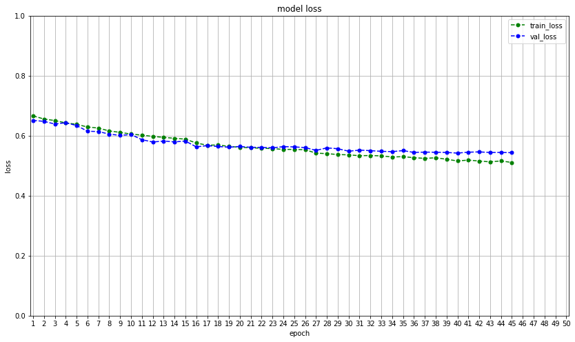
max_loss = max(max(history.history["loss"]), max(history.history["val_loss"]))
# summarize history for loss
plt.figure(figsize=(14, 8))
plt.plot(history.history["loss"], color="g", linestyle="dashed", marker="o", markerfacecolor="g", markersize=5)
plt.plot(history.history["val_loss"], color="b", linestyle="dashed", marker="o", markerfacecolor="b", markersize=5)
plt.title("model loss")
plt.ylabel("loss")
plt.xlabel("epoch")
plt.legend(["train_loss", "val_loss"]) #, loc="upper left")
plt.xlim(-.25, (max(lbl_org) + 0.25))
plt.xticks(lbl_org, lbl_new)
if max_loss <= 1:
plt.ylim(0,1)
else:
plt.ylim(0, (max_loss + (max_loss *.1)))
plt.grid()
plt.savefig("last_model_run/model loss")
plt.show()
plt.close()
# Manual test
counter = 0
for i in range(len(y_pred)):
    if y_test_expt[i] == y_pred[i]:
        counter += 1

print(counter)
print(len(y_pred))
round((counter / len(y_pred)), 4)
2133
3197


0.6672
prediction = model.predict_classes([prepare_img("test/evan_l.jpeg")])
pro = model.predict_proba([prepare_img("test/evan_l.jpeg", show=False)])
print(f"Class: {categories[prediction[0]]} {max(pro[0][0], pro[0][1]):.5%}")

Class: Normal 100.00000%
prediction = model.predict_classes([prepare_img("test/evan_f.jpeg")])
pro = model.predict_proba([prepare_img("test/evan_f.jpeg", show=False)])
print(f"Class: {categories[prediction[0]]} {max(pro[0][0], pro[0][1]):.5%}")

Class: Normal 100.00000%
prediction = model.predict_classes([prepare_img("test/not-evan_l.png")])
pro = model.predict_proba([prepare_img("test/not-evan_l.png", show=False)])
print(f"Class: {categories[prediction[0]]} {max(pro[0][0], pro[0][1]):.5%}")

Class: Normal 100.00000%
prediction = model.predict_classes([prepare_img("test/not-evan_f.png")])
pro = model.predict_proba([prepare_img("test/not-evan_f.png", show=False)])
print(f"Class: {categories[prediction[0]]} {max(pro[0][0], pro[0][1]):.5%}")
Class: Normal 100.00000%
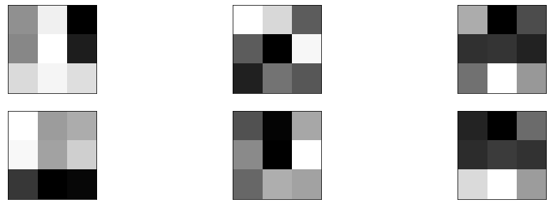
plt.figure(figsize=(16, 16))
# retrieve weights from the second hidden layer
filters, biases = model.layers[0].get_weights()
# normalize filter values to 0-1 so we can visualize them
f_min, f_max = filters.min(), filters.max()
filters = (filters - f_min) / (f_max - f_min)
# plot first few filters
n_filters, ix = 6, 1
for i in range(n_filters):
    # get the filter
    f = filters[:, :, :, i]
    # plot each channel separately
    for j in range(1):
        # specify subplot and turn of axis
        ax = plt.subplot(n_filters, 3, ix)
        ax.set_xticks([])
        ax.set_yticks([])
        # plot filter channel in grayscale
        plt.imshow(f[:, :, j], cmap='gray')
        ix += 1
# show the figure
plt.show()
counter = 0
img_path = "test/evan_l.jpeg"  # dog
# Define a new Model, Input= image
# Output= intermediate representations for all layers in the
# previous model after the first.
successive_outputs = [layer.output for layer in model.layers[1:]]
#visualization_model = Model(img_input, successive_outputs)
visualization_model = Model(inputs=model.input, outputs=successive_outputs)
# Load the input image
img = load_img(img_path, color_mode="grayscale", target_size=(128, 128))
# Convert ht image to Array of dimension (150,150,3)
x = img_to_array(img)
x = x.reshape((1,) + x.shape)
# Rescale by 1/255
x /= 255.0
# Let's run input image through our vislauization network
# to obtain all intermediate representations for the image.
successive_feature_maps = visualization_model.predict(x)
# Retrieve are the names of the layers, so can have them as part of our plot
layer_names = [layer.name for layer in model.layers]
for layer_name, feature_map in zip(layer_names, successive_feature_maps):
    print(feature_map.shape)
    if len(feature_map.shape) == 4:
        counter += 1

        # Plot Feature maps for the conv / maxpool layers, not the fully-connected layers

        n_features = feature_map.shape[-1]  # number of features in the feature map
        # feature map shape (1, size, size, n_features)
        size = feature_map.shape[1]

        # We will tile our images in this matrix
        display_grid = np.zeros((size, size * n_features))

        # Postprocess the feature to be visually palatable
        for i in range(n_features):
            x = feature_map[0, :, :, i]
            x -= x.mean()
            x /= x.std()
            x *= 64
            x += 128
            x = np.clip(x, 0, 255).astype('uint8')
            # Tile each filter into a horizontal grid
            display_grid[:, i * size: (i + 1) * size] = x
        # Display the grid
        scale = 20. / n_features
        plt.figure(figsize=(scale * n_features, scale))
        plt.title(layer_name)
        plt.grid(False)
        plt.imsave(f"last_model_run/evan{counter}.png", display_grid)
        plt.imshow(display_grid, aspect='auto', cmap='gray')
(1, 32, 32, 32)
(1, 32, 32, 32)
(1, 32, 32, 64)
(1, 8, 8, 64)
(1, 8, 8, 64)
(1, 8, 8, 64)


<ipython-input-33-c6e971e4cc9f>:39: RuntimeWarning: invalid value encountered in true_divide
  x /= x.std()


(1, 2, 2, 64)
(1, 2, 2, 64)
(1, 256)
(1, 512)
(1, 512)
(1, 256)
(1, 2)


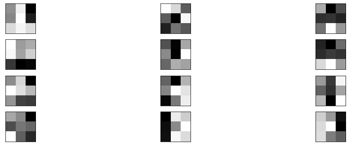
#Iterate thru all the layers of the model
for layer in model.layers:
    if 'conv' in layer.name:
        print(f"Conv:{layer.name}")
        plt.figure(figsize=(16, 16))
        # retrieve weights from the second hidden layer
        filters, biases = model.layers[0].get_weights()
        # normalize filter values to 0-1 so we can visualize them
        f_min, f_max = filters.min(), filters.max()
        filters = (filters - f_min) / (f_max - f_min)
        # plot first few filters
        n_filters, ix = 12, 1
        for i in range(n_filters):
            # get the filter
            f = filters[:, :, :, i]
            # plot each channel separately
            for j in range(1):
                # specify subplot and turn of axis
                ax = plt.subplot(n_filters, 3, ix)
                ax.set_xticks([])
                ax.set_yticks([])
                # plot filter channel in grayscale
                plt.imshow(f[:, :, j], cmap='gray')
                ix += 1
        # show the figure
        plt.show()
Conv:conv2d_1

Conv:conv2d_2

Conv:conv2d_3
loaded_model = load_model(checkpoint_filepath)
#model.save(Best_model_path)
loaded_y_pred = loaded_model.predict_classes(X_test)
prediction = loaded_model.predict_classes([prepare_img("test/evan_l.jpeg")])
pro = loaded_model.predict_proba([prepare_img("test/evan_l.jpeg", show=False)])
print(f"Class: {categories[prediction[0]]} {max(pro[0][0], pro[0][1]):.5%}")
Class: Normal 100.00000%
prediction = loaded_model.predict_classes([prepare_img("test/evan_f.jpeg")])
pro = loaded_model.predict_proba([prepare_img("test/evan_f.jpeg", show=False)])
print(f"Class: {categories[prediction[0]]} {max(pro[0][0], pro[0][1]):.5%}")
Class: Normal 100.00000%
prediction = loaded_model.predict_classes([prepare_img("test/not-evan_f.png")])
pro = loaded_model.predict_proba([prepare_img("test/not-evan_f.png", show=False)])
print(f"Class: {categories[prediction[0]]} {max(pro[0][0], pro[0][1]):.5%}")

Class: Normal 100.00000%
prediction = loaded_model.predict_classes([prepare_img("test/not-evan_l.png")])
pro = loaded_model.predict_proba([prepare_img("test/not-evan_l.png", show=False)])
print(f"Class: {categories[prediction[0]]} {max(pro[0][0], pro[0][1]):.5%}")
Class: Normal 100.00000%


Leave a comment